Another View on Context Parallel: Balancing Compute

Context Parallelism (CP) splits a batch along the sequence-length dimension, allowing each CP rank to process only a chunk of the original sequence and reducing the memory required for training.¹

Two of my favorite resources motivate CP in terms of long sequences:

Self-Attention, which is the key component of Transformers, suffers from quadratic memory requirements with respect to the sequence length, therefore when sequence length gets to a certain length, even a batch size of 1 might not be able to fit onto a single GPU and require additional partitioning along the sequence dimension. And once this is done, the sequence can be of any length.

— stas00/ml-engineering

Context Parallelism (CP) specifically targets the challenge of training with very long sequences by sharding activations along the sequence dimension across GPUs. […] CP is particularly valuable when scaling to extreme sequence lengths (128k+ tokens) where, even when using full activation recomputation, the memory requirements for attention would be prohibitive on a single GPU.

— The Ultra-Scale Playbook

That is all true, but CP has another substantial benefit: it can balance attention compute across Data Parallel ranks and improve end-to-end training time by reducing the variance of Flash Attention execution time.

The benefit comes from keeping the global batch size fixed. As CP increases, the number of DP groups decreases, so each remaining group processes proportionally more independent samples. Their attention costs are averaged across CP ranks, reducing variation.

This article gives a simple proof, a computational simulation, and a benchmark using a real Flash Attention 3 kernel on an H100.

Load balancing is important

In distributed training, iteration time is determined by the slowest rank. Even with Tensor, Pipeline, or Context Parallelism, gradients eventually have to be synchronized across Data Parallel groups. If one group reaches an all-gather or reduce-scatter later than the others, everybody else waits.

Stragglers can arise from a throttled GPU, a slow network link, or compute imbalance. Most blocks in a standard transformer scale linearly with sequence length, but attention remains quadratic. Consequently, even small fluctuations in sample length can create severe timing differences across ranks.

Ulysses

DeepSpeed Ulysses is one of the most widely adopted CP algorithms. It starts with the sequence split into \(\mathrm{CP}\) equal chunks. Before attention, an all-to-all changes the layout from sequence-sharded to head-sharded: each rank receives the full sequence for a subset of attention heads. A reverse all-to-all restores the sequence-sharded layout afterward.

This reduces per-rank activation memory by a factor of \(\mathrm{CP}\), although the exact reduction depends on the attention architecture. With GQA, KV heads may need to be replicated once CP exceeds the number of KV heads.

Theory

Problem setting

Let:

• \(\mathrm{CP}\) be the Context Parallel group size;
• \(N\) be the total device count, giving \(N/\mathrm{CP}\) independent DP/CP groups;
• \(H\) be the number of attention heads; and
• \(S\) be the token budget processed by one GPU before CP is applied.

We assume independent samples drawn from a length distribution. As CP increases, we increase the micro-batch size—and hence the token budget of each remaining group—so the global batch remains fixed:

The approximate number of independent samples processed by one group is

Since \(S/\mathbb E[L]\) is constant, let

This assumes independent samples and ignores cross-sample packing correlation.

We model Flash Attention time as quadratic in sequence length and linear in the local query-head count. For causal attention, the exact pair count is \(L(L+1)/2\), but its constant factor can be absorbed. Since Ulysses gives each rank \(H/\mathrm{CP}\) query heads,

where \(\gamma\) depends on the GPU, head dimension, and Flash Attention version.

Mean, variance, and coefficient of variation

Let \(R_i=L_i^2\) be i.i.d., with mean \(\mu_R\) and variance \(\sigma_R^2\). We require \(L\) to have a finite fourth moment.

First, the mean is constant:

For the variance,

Using (1),

Therefore,

Exponential vs. Normal distributions

The absolute variance depends heavily on the sample-length distribution. Compare:

• \(L\sim\operatorname{Exp}(\lambda)\), where \(p(L)=\lambda e^{-\lambda L}\);
• \(L\sim\mathcal N(\mu,\sigma^2)\).

Assume both have mean \(\mu=1/\lambda\), and \(\sigma\) is small enough that negative lengths are negligible. Since

we only need to compare \(\operatorname{Var}(L^2)\).

Exponential

For \(\mathbb E[L^n]=n!/\lambda^n\),

Normal

For a normal random variable,

Ratio

Let \(\mathrm{CV}=\sigma/\mu\). The ratio becomes

This gives:

• \(\mathrm{CV}=1\): \(3.33\times\);
• \(\mathrm{CV}=0.5\): \(17.78\times\);
• \(\mathrm{CV}=0.25\): \(77.58\times\);
• \(\mathrm{CV}=0.1\): \(497.51\times\).

For a tight normal distribution, variation in attention times is almost nonexistent compared with a right-skewed exponential distribution. Better data packing can therefore improve load balance. A dataset mixing many short samples with a few very long ones has a heavy right tail, dramatically increasing variance and potentially slowing each iteration.

Computational simulation

We validate the result first with a quadratic cost model, then with a real kernel. Samples are packed into a token budget of 8192; a sample crossing the boundary is split, with its remainder used in the next batch.

import numpy as np

MAX_SEQ_LEN = 8192

def read_sample():
    return min(int(np.random.exponential(MAX_SEQ_LEN // 8)), MAX_SEQ_LEN)

def read_batches(batch_size: int, n_batches: int):
    saved_sample = None
    batches = []
    for _ in range(n_batches):
        batch, current_size = [], 0
        while current_size < batch_size:
            sample = saved_sample if saved_sample is not None else read_sample()
            saved_sample = None
            if current_size + sample > batch_size:
                take = batch_size - current_size
                saved_sample, sample = sample - take, take
            current_size += sample
            batch.append(sample)
        batches.append(batch)
    return batches

def compute_flash_cost(batch: list[int]) -> float:
    return sum(s * s for s in batch)

def simulate(dp: int, cp: int, n_steps: int = 100) -> np.ndarray:
    groups = dp // cp
    local_seqlen = cp * MAX_SEQ_LEN  # keep global batch fixed
    costs = []
    for _ in range(n_steps):
        batches = read_batches(local_seqlen, groups)
        costs.append([compute_flash_cost(b) / cp for b in batches])
    return np.array(costs)

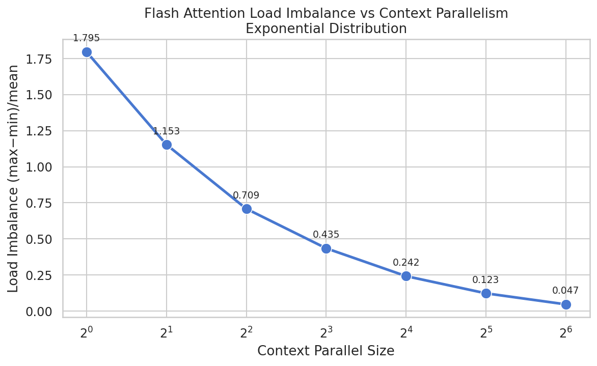
We define imbalance as \((\max-\min)/\operatorname{mean}\) across DP groups.

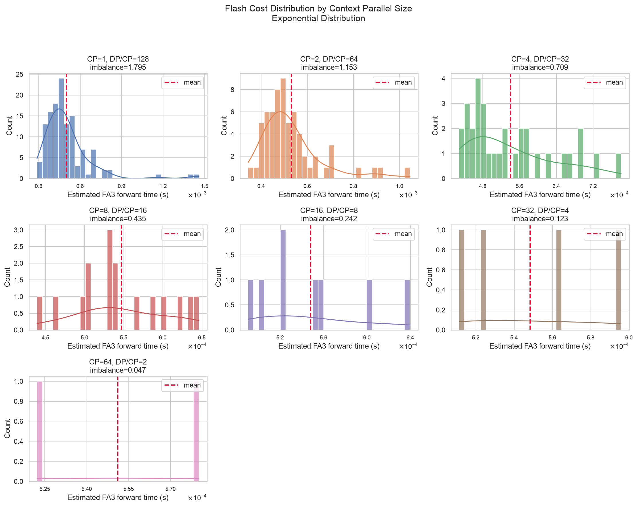
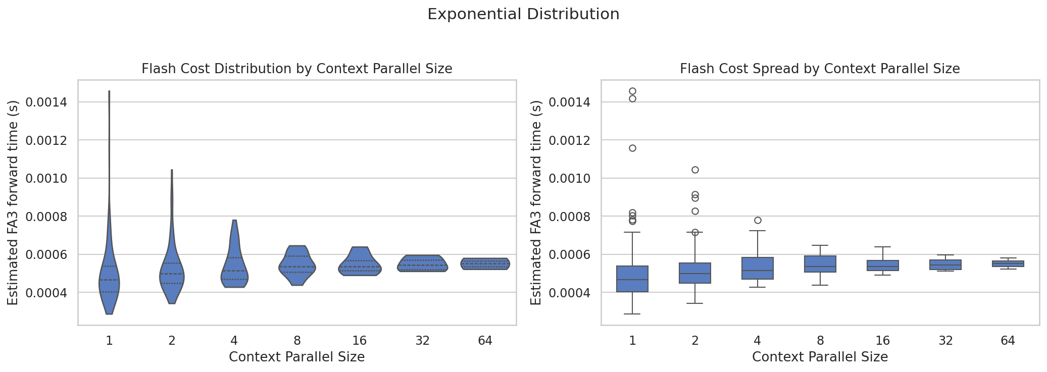
With \(\mathrm{CP}=1\), the maximum time is seven times the minimum. With \(\mathrm{CP}=8\), the max-to-min ratio is less than two.

Benchmarking real kernels

Following my CUDA benchmarking guide, I benchmarked Flash Attention 3 on a single H100. I used \(\mathrm{DP}=128\), a base sequence length of 8192, and scaled the micro-batch size linearly with CP.

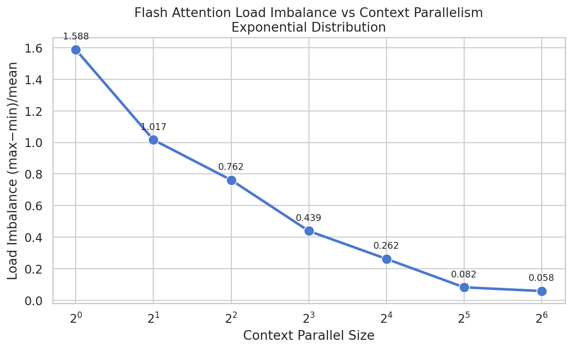
The measured results align almost ideally with the theoretical prediction.

Results

Context Parallelism provides an excellent opportunity to balance load across ranks. Other approaches include packing batches beforehand or avoiding heavy-tailed data distributions, but CP provides a strong and simple baseline.

Many CP implementations add communication that is too slow or too difficult to overlap. So while setting \(\mathrm{CP}=\mathrm{DP}\) is possible, it may make sense only for certain variants, such as Magi Attention.

Code

The full simulation source is available on GitHub. You can rerun it with your own data distribution, DP count, and other parameters.